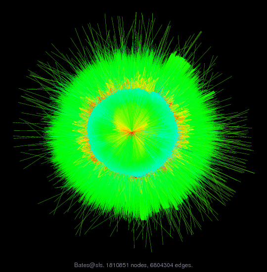
Matrix: Bates/sls
Description: Large least-squares problem (GPA) Doug Bates, Univ of Wisconsin-Madison
 |
| (bipartite graph drawing) |
 |
| Matrix properties | |
| number of rows | 1,748,122 |
| number of columns | 62,729 |
| nonzeros | 6,804,304 |
| structural full rank? | yes |
| structural rank | 62,729 |
| # of blocks from dmperm | 1 |
| # strongly connected comp. | 1 |
| explicit zero entries | 0 |
| nonzero pattern symmetry | 0% |
| numeric value symmetry | 0% |
| type | real |
| structure | rectangular |
| Cholesky candidate? | no |
| positive definite? | no |
| author | D. Bates |
| editor | T. Davis |
| date | 2008 |
| kind | least squares problem |
| 2D/3D problem? | no |
Notes:
Large least-squares problem from Doug Bates, Univ of Wisconsin-Madison

http://www.stat.wisc.edu/~bates

The data are 10 years of grade point scores at a large state
university (not mine).  The covariates that are recorded with the
scores are the student id, the instructor id and the department.

Number of obs: 1685394, groups: id, 54711; instr, 7915; dept, 102

Even though these scores are from different semesters and one of the
questions of interest is whether grade inflation has taken place,
initially I fit a simple model that has an effect for the student, an
effect for the instructor and an effect for the department.  There is
also an overall average gradepoint.  The overall average is what we
call a fixed effect. In computations terms this means it is estimated
without a penalty. The other effects are what we call random effects.
In terms of parameters we estimate a variance for each group of random
effects (student, instructor and department).  We assume that the
random effects come from a normal (or Gaussian) distribution, which
has the effect of shrinking the estimates of the individual effects
towards the origin.  If the variance of that distribution is large,
there is little penalty and the estimates for each of the students or
each of the instructors or each of the departments is close to the
least squares estimate.  If the variance is small then they are much
closer to zero.

Overall we will estimate 3 variances, 1 fixed-effect and 62728 = 54711
+ 7915 + 102 random effects. The matrix we will decompose will be
62729 columns (the last column comes from the fixed-effect) and
1685394 + 62728 rows.  The 62728 rows come from the penalty part and
consist of an identity matrix of size 62728 with a column of zeros
appended on the right.  The rows determined by the data (I think of
these as being the top part of the matrix but it doesn't matter if
they are on the top or the bottom) consist of 54711 columns of
indicators for the student followed by 7915 columns of indicators for
the instructor followed by 102 columns of indicators for the
department followed by a column of 1's.  In general we will have
columns for random effects followed by columns for fixed effects.
Here the fixed-effects column is trivial but in general we may have
more than 1 and they don't have to be as trivial as this.

At least as far as I have been able to analyze the computation, I can
allow for permutations of the columns for the random effects but I
don't want to mix up the columns for the random effects and the
columns for the fixed effects. I always want to keep the columns for
the fixed effects as a block on the right. (Usually these columns are
dense or close to it so it isn't a problem to force them to be on the
right.) The reason is that I need the logarithm of the square of the
determinant of the triangular factor from the random effects columns
only.

During the optimization phase we fix values of the three variances,
update the numeric values in the matrix, decompose, calculate the
determinant of the leading part of the triangular factor, and evaluate
the penalized residual sum of squares.  The logarithm of the
determinant and the penalized residual sum of squares are combined to
create a criterion called the profiled log-likelihood which is to be
maximized

The update operation changes the numerical values of the
data-determined part according to three multipliers.  The first
multiplier is applied to the first 54711 columns, the next multiplier
is applied to the next 7915 columns and the last multiplier is applied
to the next 102 columns.  The last column stays fixed.

We start from the factors for the student, instructor and department
then generate the indicators to form Z.  The factors can be
represented as integers and the response is a grade point score
(allowed to be half integers).
| Ordering statistics: | result |
| nnz(V) for QR, upper bound nnz(L) for LU, with COLAMD | 9,317,956,486 |
| nnz(R) for QR, upper bound nnz(U) for LU, with COLAMD | 25,472,608 |
For a description of the statistics displayed above, click here.
Maintained by Tim Davis, last updated 12-Mar-2014.
Matrix pictures by cspy, a MATLAB function in the CSparse package.
Matrix graphs by Yifan Hu, AT&T Labs Visualization Group.