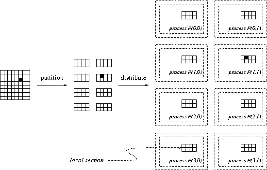
Figure 2 illustrates how data for a 2-dimensional mesh computation is distributed over a 2-dimensional grid of processes: The original (undistributed) 16-by-16 array is partitioned into contiguous subarrays (called local sections) and distributed among a 4-by-2 grid of processes.
Observe that now each element in the array has two sets of indices -- its global indices (reflecting its position in the original undistributed array) and its local indices (reflecting its position in the local section). (For example, using the Fortran convention of starting array indices at 1, the shaded square has global indices (3,6) and local indices (1,2) in the grid process (2,1).)